Author’s note: if you like this post, you might like Landmark Atlas. This is my new blog where I tell stories about Britain’s history, culture and geography through maps.
In a previous post I showed how to access and plot data from Open Street Map (OSM) in R. When I started my mapping project OSM was the data source I used. After I discovered Ordnance Survey’s (OS) open data, I switched over to theirs instead.
In this post I’ll explain how to get hold of the OS data and plot it using R. The code is here on GitHub.
Ordnance Survey open data
OS is a mapping agency for Great Britain. They publish all kinds of topographical data about Britain such as addresses, roads, terrain, contours and more besides.
I had always assumed OS data was a paid-for service. They publish various paid-for datasets but they also have a rich source of open data available to download.
Grid squares
Fundamental to understanding OS data is the concept of grid references. These are squares 100km by 100km that divide up the island of Great Britain.
Some OS open data covers the whole of Britain while other datasets allow you to choose a grid square or squares to save you having to download data you don’t need.
Accessing OS data
In this post I’m going to show you how to download OS data and use it to plot a simple map of the Isle of Mull in the Hebrides, Scotland.
We’re going to start with the VectorMap District data. Head to that link, choose ‘Set a custom area’ and choose the NM grid square. Choose ESRI shapefile and download.

Extract the data and put it in a folder called os-walkthrough in your working directory.
Looking inside the folder, you can see there are various shapefiles representing different features in the NM grid square.

We’re going to plot roads, rivers, bodies of water and forests. Load all of these shapefiles using the following commands:
wood <- read_sf('path/to/folder/data/NM_Woodland.shp') %>% st_transform(4326)

roads <- read_sf('path/to/folder/NM/data/NM_Road.shp') %>% st_transform(4326)

water <- read_sf('path/to/folder/NM/data/NM_SurfaceWater_Area.shp') %>% st_transform(4326)

rivers <- read_sf('path/to/folder/NM/data/NM_SurfaceWater_Line.shp') %>% st_transform(4326)
Note that we are transforming these shapefiles into the WGS 84 coordinate reference system (CRS).
Putting the backdrop in place
This is a plot of these features centred around the Isle of Mull in Scotland.
coords <- matrix(c(-6.49,-5.6,56.245,56.668), byrow = TRUE, nrow = 2, ncol = 2, dimnames = list(c('x','y'),c('min','max')))|

ggplot() +
     geom_sf(data = wood, fill = '#4F9638', color = NA) +
     geom_sf(data = water, fill = '#cce6ff', color = NA) +
     geom_sf(data = rivers, fill = '#cce6ff', color = NA) +
     geom_sf(data = roads, fill = '#B4BFB0',color = '#B4BFB0') +
     theme_minimal() +
     coord_sf(xlim = c(coords[1], coords[1,2]),
            ylim = c(coords[2], coords[2,2]),
            expand = FALSE)

We can see that the forest and shore have come out nicely. The problem is that there is no distinction in the plot between land and sea.
As ever with R, there are a number of solutions to this. A simple one is to plot a country shapefile of the whole of Scotland as a backdrop.
To do this, head to the ONS Geography geoportal page and download the countries 2019 shapefile.

Load the shapefile in the usual way and narrow it down to Scotland.
shp <- read_sf('path/to/country/shapefile/Countries__December_2019__Boundaries_UK_BFC.shp')
scotland <- shp[shp$ctry19nm == 'Scotland',]
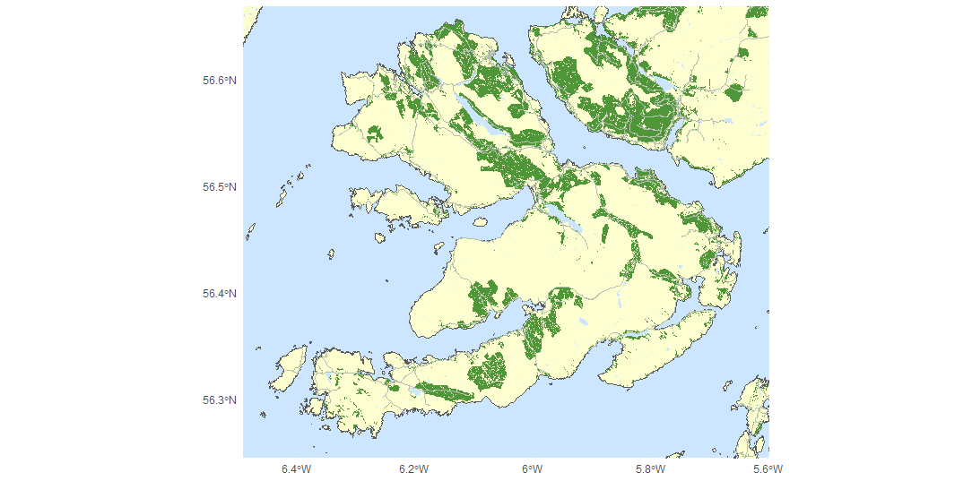
We will add a blue rectangle as a base to represent the sea and then plot the land and features on top of that.
The order in which you plot features is very important when working with geospatial data. A good rule of thumb is to plot natural features first and man-made ones on top. In other words, whatever was there ‘first’ should be plotted first, so that features that appeared later will appear overlaid on top.
ggplot() + geom_rect(data = scotland, mapping=aes(xmin=coords[1], xmax=coords[1,2], ymin=coords[2], ymax=coords[2,2]), fill= '#cce6ff') +
   geom_sf(data = scotland, fill = '#fdffd0') +
   geom_sf(data = wood, fill = '#4F9638', color = NA) +
   geom_sf(data = water, fill = '#cce6ff', color = NA) +
   geom_sf(data = rivers, fill = '#cce6ff', color = NA) +
   geom_sf(data = roads, fill = '#B4BFB0',color = '#B4BFB0') + theme_minimal() +
   coord_sf(xlim = c(coords[1], coords[1,2]),
   ylim = c(coords[2], coords[2,2]),
   expand = FALSE)

There are obviously more features that you could add. As a quick base map it’s a great start.
Conclusion
This was a tutorial of how to draw a large rural area using OS data.
This technique is different from how to draw a small, densely-populated urban area. That technique deserves its own post to follow.