Introduction
NHS England has started to publish data on the numbers of COVID-19 vaccination doses it has carried out on people in England.
These weekly spreadsheets contain lots of very useful data with different breakdowns. The one we’re interested in is the data broken down by Middle Layer Super Output Area (MSOA).
MSOAs are roughly equivalent to ‘neighbourhoods’. They carry names that are recognisable to local residents and are home to around 7,200 people each.
I decided to build on Claire Miller’s (my former colleague) work mapping this data. I’ve turned it into an interactive tool so users can the progress being made on COVID-19 vaccinations in your area.
The full code for the R script and the accompanying Shiny app are on GitHub.
Getting the data and shapefile
There are three sources of data we will need for this piece of work:
Download the files from these locations and put them in your working directory. Unzip them if necessary. Use the mid-2019 data for the population estimates. Make sure you include all six files that come with the shapefile.
We’re going to make use of the readxl package, which is part of the tidyverse and the sf package to load these files in.
library(tidyverse)
library(sf)
library(shiny)
library(devtools)
devtools::install_github("yutannihilation/ggsflabel")
library(ggsflabel)

vacc <- readxl::read_xlsx('COVID-19-weekly-announced-vaccinations-4-March-2021-1.xlsx', sheet = 'MSOA', skip = 14, col_names = FALSE)

#add new col names
names(vacc) <- c('region_code','region_name','LA_code','LA_name','MSOA_code','MSOA_name','Under 65','65-69','70-74','75-79','80+')

#get shapefile
msoa_detailed <- read_sf('Middle_Layer_Super_Output_Areas__December_2011__Boundaries_EW_BFE.shp')

#read in population
msoa_pop <- readxl::read_xlsx('SAPE22DT4-mid-2019-msoa-syoa-estimates-unformatted.xlsx', sheet = 'Mid-2019 Persons', skip = 3)
Note that when you use read_xlsx() you have to specify which sheet of the Excel file you want to read. We are using the skip argument to skip the first few lines of the sheets that introduce the data.
Getting the population aged 65 and over
The msoa_pop data frame has the population by single year of age for each MSOA. We need to sum the populations aged 65 or over for each area. A simple way to do this is to isolate the data you want and run rowSums().
Then we add back in the codes and labels so we know which is which.
#add up 65+
msoa_pop_65 <- msoa_pop[,73:98]
msoa_pop_65$total <- rowSums(msoa_pop_65)

#cut data frame to just 65+
msoa_pop_65 <- cbind(msoa_pop[,1:6], msoa_pop_65$total)
names(msoa_pop_65)[7] <- 'total_over_65'
Calculate the percentage of people vaccinated
We’ll run rowSums() again to get the total number of people aged 65 and over who have been vaccinated and then calculate the percentage vaccinated.
#add to vacc
vacc <- merge(vacc, msoa_pop_65, by.x = 'MSOA_code', by.y = 'MSOA Code')

#calc percentage
vacc$over_65_vaccinated <- rowSums(vacc[,8:11])
vacc$pc <- vacc$over_65_vaccinated / vacc$total_over_65 * 100
You may notice that some areas have a vaccination percentage over 100%.
There are a couple of reasons for why this might be:
- The ONS data are estimates, with the margin of error increasing at smaller areas like these ones.
- The data are from mid-2019 and the populations of certain areas may have grown since then.
Merge in the shapefile
vacc_shp <- merge(vacc, msoa_detailed, by.x = 'MSOA_code', by.y = 'MSOA11CD')
vacc_shp <- arrange(vacc_shp, MSOA_code)
#vacc_shp <- sf::st_transform(vacc_shp, crs = 4326)
Get the relevant dates
This is a little trick to get the period that the data covers easily. The data is updated weekly. To save hassle I’m reloading the spreadsheet, finding the cell containing the dates and saving it as a character vector.
#get date period
vacc_date <- readxl::read_xlsx('COVID-19-weekly-announced-vaccinations-4-March-2021-1.xlsx', sheet = 'MSOA')
vacc_date <- vacc_date[2,2] %>% as.character()
vacc_date <- gsub('2020 ','',vacc_date)
vacc_date <- gsub('2021','',vacc_date)
vacc_date <- trimws(vacc_date)
Choose a local authority and tidy up labels
In this section you can choose the local authority you want to plot. Our plot will label each MSOA with its name using the ggsflabel package.
A major challenge when building this app was to condense a lot of information on to a small screen. MSOA labels are often long.
There is also a wide variation in how many MSOAs are in each local authority district: Birmingham has 132 while Rutland has five.
We will account for this in two ways:
- Shorten common words such as compass points.
- Display every other label or even every fifth label for larger local authorities with more MSOAs.
#choose a LA
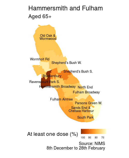
chosen_LA <- 'Hammersmith and Fulham'
df <- vacc_shp[vacc_shp$LA_name == chosen_LA ,]
df$MSOA_name <- gsub('&','&\n', df$MSOA_name)
df$MSOA_name <- gsub(' and ',' and \n', df$MSOA_name)
df$MSOA_name <- gsub(' South West',' SW.', df$MSOA_name)
df$MSOA_name <- gsub(' North West',' NW.', df$MSOA_name)
df$MSOA_name <- gsub(' South East',' SE.', df$MSOA_name)
df$MSOA_name <- gsub(' North East',' NE', df$MSOA_name)
df$MSOA_name <- gsub(' West',' W.', df$MSOA_name)
df$MSOA_name <- gsub(' East',' E.', df$MSOA_name)
df$MSOA_name <- gsub(' South',' S.', df$MSOA_name)
df$MSOA_name <- gsub(' North',' N.', df$MSOA_name)
df$MSOA_name <- gsub(' Central',' Cen.', df$MSOA_name)
df$MSOA_name <- gsub(' Junction',' Jun.', df$MSOA_name)
df$MSOA_name <- gsub('Centre','Cen.', df$MSOA_name)
df$MSOA_name <- gsub(' Road',' Rd', df$MSOA_name)
df$MSOA_name <- gsub(' Street',' St', df$MSOA_name)
df$MSOA_name <- gsub(' Lane',' Ln', df$MSOA_name)
labels <- df
if(nrow(labels) >= 25 && nrow(labels) <= 50) {
seq <- seq(1,nrow(labels),by=2)
labels$num <- seq(1,nrow(labels), by = 1)
labels <- subset(labels, num %in% seq)
} else if(nrow(labels) >=51) {
seq <- seq(1,nrow(labels),by=5)
labels$num <- seq(1,nrow(labels), by = 1)
labels <- subset(labels, num %in% seq)
}Plot
p <- ggplot() +
    geom_sf(data = df, aes(geometry = geometry, fill = pc), color = NA)   + scale_fill_distiller(palette = "YlOrBr", direction = -1, trans = 'reverse')  + labs(
      title = paste0(chosen_LA ),
      subtitle ='Aged 65+',
      fill = "At least one dose (%)",
      caption = paste0('Source: NIMS\n',vacc_date)) + theme_void(base_size = 18)+ theme(legend.position='bottom', legend.text=element_text(size=8)) + geom_sf_text_repel(data = labels, aes(label = MSOA_name), segment.colour = NA, size = 4, inherit.aes = TRUE, force = 2, ylim = c(-Inf, Inf), lineheight = .75, colour = 'black')
  p
Contains OS data © Crown copyright and database right 2020
Our plot automatically changes the title based on which area you choose. Labels are nicely sized and spaced.
To maximise use of space on small screens I’ve placed the legend underneath the plot using theme(legend.position='bottom', legend.text=element_text(size=8)).
Shiny app
I’ve wrapped this in a Shiny app which you can try at the top of this post or directly hosted on Shinyapps.io.
I had to tweak the code slightly, copying some of the ggsflabel functions directly into the code because the package is not listed on CRAN. Reading in the Excel files seemed to cause a memory problem so for the Shiny app they are saved as CSVs.
Conclusion
I’m getting faster at making Shiny apps. The RStudio Gallery has numerous examples to choose from that you can base your own apps on. I’ve found this very helpful to get started.
I’ll try to keep this app updated as the new weekly data come in.