Author’s note: if you like this post, you might like Landmark Atlas. This is my new blog where I tell stories about Britain’s history, culture and geography through maps.
What is Open Street Map?
Open Street Map (OSM) is a world map put together by volunteers. Its data is open, meaning that with appropriate credit you can use OSM data for your own work.
It has topographical features such as rivers and forests as well as man-made features such as roads and buildings.
Here is an embedded OSM map centred on central London (it may need zooming in):
View Larger Map
What are the strengths of OSM?
International
OSM covers the entire world (in varying degrees of detail). It’s unlikely that national statistics agencies for different countries will have much, if any, geospatial data that doesn’t pertain directly to them.
Open data
OSM allows you to reuse their data, including for commercial purposes, provided you credit them appropriately. This is usually as simple as putting:
© OpenStreetMap contributors
Coverage and accuracy
The map itself is usually comprehensive, meaning it doesn’t leave out any major features. It is also very accurate when you compare it to other sources of map data available online.
How do you access Open Street Map in R?
You can obtain access to OSM data in R via the osmdata package.
To get started, load the osmdata package and let’s begin drawing a map of bars in a section of central London.
We have to work with OSM’s Overpass query. The first thing to do is to specify the location in the world that we are interested in mapping using the opq() function. There are two ways to do this.
- Specify a named location
- Specify the bounding box for Open Street Map to draw. You do this with two latitude and longitude coordinates which will form the limits of your box.
The first option is the simpler one. The second one is more complex but offers more flexibility by essentially saying to Open Street Map: ‘Give me everything within this area’.
I recommend the second option if you are interested in drawing a large or densely-populated area. If you request ‘London’ OSM will give you the entire city, which may time out the server request or at any rate provide you with a lot of data that you won’t need.
#first option (not recommended in this case)
library(osmdata)
library(tidyverse)
library(sf)

town <- 'London'
location <- town %>% opq()

#second option (recommended)
coords <- matrix(c(-0.1,-0.07,51.5,51.52), byrow = TRUE, nrow = 2, ncol = 2, dimnames = list(c('x','y'),c('min','max')))
location <- coords %>% opq()
Retrieving OSM data
Open Street Map has two attributes to identify things on a map: features and tags.
A feature is a type of object that can be mapped such as buildings, highways and railways. Features contain various tags that go into more detail about what the feature is. For example the natural feature contains the likes of wood, coastline and beach.
Building a query
water <- location %>%
   add_osm_feature(key = "natural",
                   value = c("water")) %>%
   osmdata_sf()
Here is a sample query. Note that we are using the location that we defined earlier and adding the OSM feature ‘natural’ with the ‘water’ tag. Finally the osmdata_sf() function actually requests the data from the server in simple feature (sf) format, which we have been using so far in this series.
You’ll notice a c() in front of water. I put this there by default because sometimes I want to search for more than one tag e.g. value = c("water","coastline")
Examining the result
This query returns a list of different types of geospatial data:
- points
- lines
- polygons
- multipolygons
Which one is suitable to plot depends on the feature you are interested in. For individual features such as cafes or statues points may be appropriate. For roads it will likely be lines. For lakes it may be polygons or even multipolygons.
In this case it’s the multipolygons that have the best, most useable plot of the River Thames:
ggplot() + geom_sf(data = water$osm_multipolygons, fill = 'light blue') + theme_minimal()

The code below builds up a map of pubs in central London.
#build different types of streets
main_st <- data.frame(type = c("motorway","trunk","primary","motorway_junction","trunk_link","primary_link","motorway_link"))
st <- data.frame(type = available_tags('highway'))
st <- subset(st, !type %in% main_st$type)
path <- data.frame(type = c("footway","path","steps","cycleway"))
st <- subset(st, !type %in% path$type)
st <- as.character(st$type)
main_st <- as.character(main_st$type)
path <- as.character(path$type)
#query OSM
main_streets <- location %>%
add_osm_feature(key = "highway",
value = main_st) %>%
osmdata_sf()
streets <- location %>%
add_osm_feature(key = "highway",
value = st) %>%
osmdata_sf()
water <- location %>%
add_osm_feature(key = "natural",
value = c("water")) %>%
osmdata_sf()
rail <- location %>%
add_osm_feature(key = "railway",
value = c("rail")) %>%
osmdata_sf()
parks <- location %>%
add_osm_feature(key = "leisure",
value = c("park","nature_reserve","recreation_ground","golf_course","pitch","garden")) %>%
osmdata_sf()
buildings <- location %>%
add_osm_feature(key = "amenity",
value = "pub") %>%
osmdata_sf()
#plot map
ggplot() + geom_sf(data = water$osm_multipolygons, fill = 'light blue') + theme_minimal()
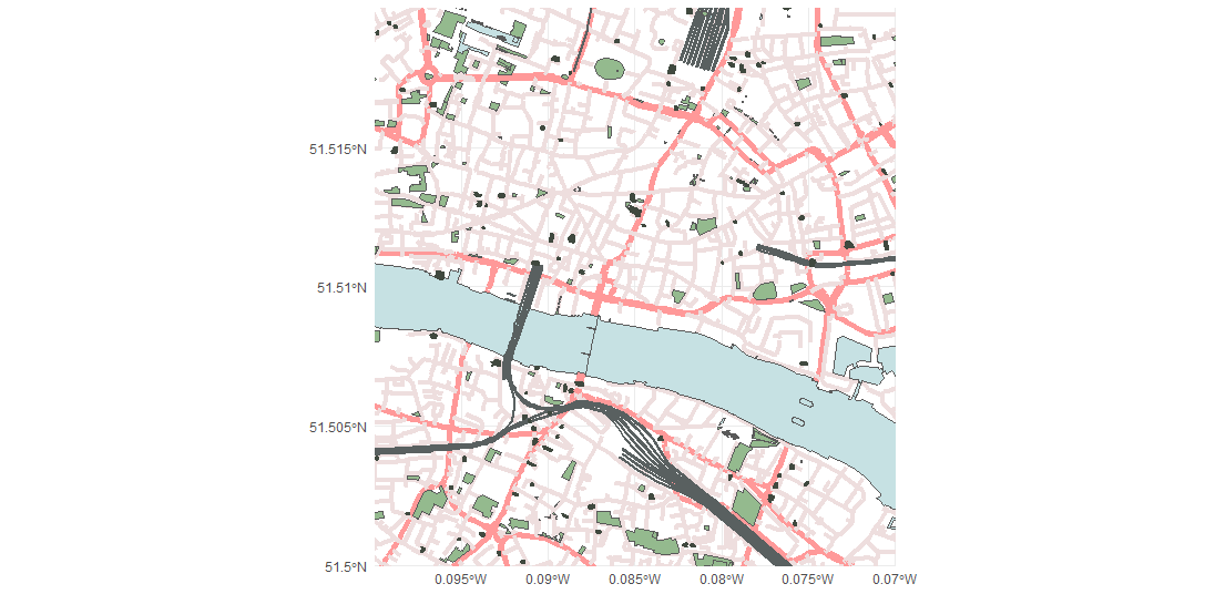
ggplot() +
geom_sf(data = main_streets$osm_lines, color = '#ff9999', size = 2) +
geom_sf(data = streets$osm_lines, size = 1.5, color = '#eedede') +
geom_sf(data = water$osm_polygons, fill = '#c6e1e3') +
geom_sf(data = water$osm_multipolygons, fill = '#c6e1e3') +
geom_sf(data = rail$osm_lines, color = '#596060', size = 1) +
geom_sf(data = parks$osm_polygons, fill = '#94ba8e') +
geom_sf(data = buildings$osm_points, color = '#40493f', fill = '#40493f', size = 2) +
coord_sf(xlim = c(coords[1], coords[1,2]),
ylim = c(coords[2], coords[2,2]),
expand = FALSE) + theme_minimal()

The pubs are the dark blobs on the map.
A few things to note about the code:
- There are lots of different options in the
highwayfeature so I made vectors calledmain_st,standpath(not pictured) to divide them up. - The
coord_sf()function allows you to specify the area to plot. This is useful because sometimes an OSM object will stretch out beyond the confines of your bounding box, like the River Thames in our earlier example. This is what the same code looks like withoutcoord_sf():

Not much good.
- The plot uses a healthy mix of points, lines, polygons and multipolygons
- The colour values are hex codes. There are numerous websites devoted to helping you pick the right one – a certain amount of trial and error is needed to get ones you are happy with.
Conclusion
That is my beginner’s overview to using Open Street Map. For more, please study the list of features and see what you can discover.
As I said in my introductory post, I started my mapping journey with Open Street Map and then moved to Ordnance Survey data. I’ll show you how to work with OS data in another post. I will also write another one comparing the pros and cons of the two sources.