A beautiful body of work emerged from the horrors of the First World War: poetry.
Poets have written and sung songs about war since antiquity. But up until the 19th century the vast majority of men who actually fought were illiterate. They could not write down their experiences, so much of it was lost to history or left to the few who could read and write, such as Shakespeare, to record.

The First World War, however, was one of the first fought in world history by troops who were almost entirely literate. Quickly the war reached a frightening, dull stalemate in the trenches, with well-educated men huddled below ground a few hundred yards from men from similar backgrounds on the other side. To pass the time, to record the horrors of 20th century warfare for posterity or simply to put into words what they were thinking, many soldiers at the front line picked up a pen and paper and recorded their experiences. Likewise, those back home could write about their husbands, sons and brothers at the front.
Much of it has been collected by the Poetry Foundation on this page. In this post we will do some textual analysis (natural language processing) of the poems using R to see whether we can pick out any themes and how they changed over the course of the war.
The full code:
library(rvest)
library(tidyverse)
library(tidytext)

setwd('your-directory')

url_list <- read_html('https://www.poetryfoundation.org/articles/70139/the-poetry-of-world-war-i')
url_list <- url_list %>% html_nodes('div.c-userContent p a') %>% html_attr('href')
url_list <- url_list[grepl('/poem/',url_list)]
url_list <- gsub('http://www.poetryfoundation.org/','',url_list)
url_list <- paste0('http://www.poetryfoundation.org/',url_list)

poem_urls <- lapply(url_list, read_html)

#define functions
get_text <- function(url) {
text <- url %>% html_nodes('div.c-feature-bd div') %>% html_text()
text <- text[!grepl('Poetry Out Loud Note',text)]
text <- paste(text[!grepl('\n',text)], collapse = ' ')
}

get_title <- function(url) {
title <- url %>% html_nodes('div.c-feature-hd h1') %>% html_text()
title <- title[1]
}

get_author <- function(url) {
author <- url %>% html_nodes('div span') %>% html_text()
author <- author[grepl('By ',author)][1]
author <- gsub('\n ','',author)
author <- trimws(gsub('By ','',author))
}

results <- data.frame(text = as.character(lapply(poem_urls, get_text)),
title = as.character(lapply(poem_urls, get_title)),
author = as.character(lapply(poem_urls, get_author)),
url = url_list, stringsAsFactors = FALSE)

results$year <- NA
results$year[1:14] <- 1914
results$year[15:32] <- 1915
results$year[33:49] <- 1916
results$year[50:67] <- 1917
results$year[68:82] <- 1918
results$year[83:101] <- '1919-28'

words <- results %>% unnest_tokens('word','text')
words <- words %>% anti_join(stop_words)

#analysis
word_count <- words %>%
group_by(word, year) %>%
summarise(count = n())

word_count <- word_count %>% spread(key = 'year', value = 'count', fill = 0)
word_count$total <- rowSums(word_count[,2:7])

#filter to 15
word_count <- word_count[word_count$total >= 15, 1:7]
word_count <- gather(word_count, 'year','total',-word)

ggplot(word_count, aes(x = reorder(str_to_title(word), desc(word)), y = total, group = year, fill = year)) +
facet_grid(cols = vars(year)) + theme_minimal() +
geom_col() + coord_flip() +
theme(legend.position = 'none',
panel.grid.minor.x = element_blank(),
panel.grid.major = element_line(color = '#BABABA')) +
scale_fill_manual(values = c('#F79090','#F86F6F','#EA3030','#C82222','#9B1111','#6C0707')) +
labs(title = 'Most common words mentioned in First World War poetry, by year',
y = 'Count of mentions',x = '',
caption = 'Source: Analysis of WW1 poetry at poetryfoundation.org')

ggsave('ww1_poetry.png',last_plot(),width = 9.5, height = 7.8)
Step 1, load packages:
Install the relevant packages and load them. We need tidyverse for data analysis, rvest for scraping and tidytext for the text analysis.
Step 2, get the list of poems:
library(rvest)
library(tidyverse)
library(tidytext)

setwd('your-directory')
Step 3, get the URLs to scrape:
url_list <- read_html('https://www.poetryfoundation.org/articles/70139/the-poetry-of-world-war-i')

#collect the URLs from the page
url_list <- url_list %>% html_nodes('div.c-userContent p a') %>% html_attr('href')

#tidy up URLs
url_list <- url_list[grepl('/poem/',url_list)]
url_list <- gsub('http://www.poetryfoundation.org/','',url_list)
url_list <- paste0('http://www.poetryfoundation.org/',url_list)
Often scraping is a two or even three-step process. The first of these is to scrape (or generate) the URLs you want. In this case we will scrape the URLs from the page. Some of them are published in journals and won’t be possible to scrape, so we will leave those. Others need tidying up as some have the poetryfoundation.org prefix in front of them and some don’t.
Step 4, read the URLs:
poem_urls <- lapply(url_list, read_html)
The downside of scraping in R compared to a program like OutWit Hub is that it can take a while to read all the URLs you want to scrape. This step takes a while, so put the kettle on.
Step 5, define the functions:
#define functions
get_text <- function(url) {
text <- url %>% html_nodes('div.c-feature-bd div') %>% html_text()
text <- text[!grepl('Poetry Out Loud Note',text)]
text <- paste(text[!grepl('\n',text)], collapse = ' ')
}

get_title <- function(url) {
title <- url %>% html_nodes('div.c-feature-hd h1') %>% html_text()
title <- title[1]
}

get_author <- function(url) {
author <- url %>% html_nodes('div span') %>% html_text()
author <- author[grepl('By ',author)][1]
author <- gsub('\n ','',author)
author <- trimws(gsub('By ','',author))
}
As I said earlier, scraping is usually a multi-step process. Now that we have the URLs we want in a format to scrape, we can define what we actually want from them.
These three functions get the text, the author and the title from the URLs. We will apply these functions later. The advantage of doing this is that you can do much of the data cleaning in the scraping process.
For example:
author <- read_html('https://www.poetryfoundation.org/poems/57420/elegy-in-a-country-courtyard') %>% html_nodes('div span') %>% html_text()
> author
[1] "\n Show Menu\n \n "
[2] "Show Menu"
[3] ""
[4] "Poetry Foundation"
[5] ""
[6] "\n By G. K. Chesterton\n "
[7] "\n Source:\n The Ballad of St. Barbara and Other Poems\n (1922)\n "
[8] "More Poems by G. K. Chesterton"
[9] "By G. K. Chesterton"
[10] "By G. K. Chesterton"
[11] "By G. K. Chesterton"
[12] "By G. K. Chesterton"
[13] "By G. K. Chesterton"
[14] "Poetry Foundation Children"
[15] "Poetry Magazine"
[16] "61 West Superior Street, Chicago, IL 60654"
[17] "Hours: Monday-Friday 11am - 4pm"
[18] "\n By G. K. Chesterton\n "
[19] "\n About this Poet\n "
[20] "More About this Poet"
[21] "Region:"
[22] "School/Period:"
[23] "Quick Tags"
Here is what the scraper brings back initially. The author’s name is in there, several times, as ‘By G.K. Chesterton’.
> author <- author[grepl('By ',author)][1]
> author
[1] "\n By G. K. Chesterton\n "
Running this grepl command narrows it down to one, with some redundant line spaces and a ‘by’.
> author <- gsub('\n ','',author)
> author <- trimws(gsub('By ','',author))
> author
[1] "G. K. Chesterton"
Bingo. Including all of this in the function gets this out of the way early so we can collect the results neatly.
It can be a bit of trial and error to work out exactly what element of the page you want to scrape. For more information on how to find the needles in the HTML haystack, see this post I did on scraping.
Step 6, collect the results:
results <- data.frame(text = as.character(lapply(poem_urls, get_text)),
title = as.character(lapply(poem_urls, get_title)),
author = as.character(lapply(poem_urls, get_author)),
url = url_list, stringsAsFactors = FALSE)

results$year <- NA
results$year[1:14] <- 1914
results$year[15:32] <- 1915
results$year[33:49] <- 1916
results$year[50:67] <- 1917
results$year[68:82] <- 1918
results$year[83:101] <- '1919-28'
Now we can collect our results in a nice neat data frame by using lapply to apply our custom functions to each scraped URL.
One variable we didn’t collect in the scrape was the year of publication. I decided to do this manually because of the way the Poetry Foundation poems list is laid out.
Step 7, split into words:
words <- results %>% unnest_tokens('word','text')
words <- words %>% anti_join(stop_words)
Much text analysis begins at the level of the individual word. What are the most common words to appear in a book? Do words carry a positive or negative connotation?
To analyse the words in a book or poem you need to separate them out individually first. We can do this using unnest_tokens from the tidytext package. This splits sentences and paragraphs into individual words. Crucially it also retains the other variables from the text, in our case keeping the poem, year and author.
Secondly, the package has a handy list of stop words. These are common prepositions, articles and pronouns like ‘and’, ‘I’ or ‘about’ that are essential in English but don’t convey much in the way of meaning. Running the anti_join function removes these words from our data frame.
Step 8, word count:
#analysis
word_count <- words %>%
group_by(word, year) %>%
summarise(count = n())

word_count <- word_count %>% spread(key = 'year', value = 'count', fill = 0)
word_count$total <- rowSums(word_count[,2:7])
Now we are going to find out the most common words by doing a count. We will group_by year as well to find out the most common words by year. Having done that, we will use spread to push this vertical data into horizontal data, with columns for each year. Then we will use rowSums to work out an overall total for each word across the entire era.
Step 9: Filter for the most common words
#filter to 15
word_count <- word_count[word_count$total >= 15, 1:7]
>word_count
# A tibble: 57 x 7
# Groups:   word [57]
   word   `1914` `1915` `1916` `1917` `1918` `1919-28`
   <chr>   <dbl>  <dbl>  <dbl>  <dbl>  <dbl>     <dbl>
 1 air         1      2      3      3      2         5
 2 beauty      0      8      1      3      1         4
 3 blind       3      3      2      5      2         0
 4 blood       1      3      2      8      5         5
 5 bright      1      5      3      3      1         3
 6 cold        2      3      4      0      4         2
 7 dark        1      1      2     12      3         3
 8 day         9     10      4      6      7        10
 9 days        0      3      2      1      4         5
10 dead        2      9     17     18      6        11
# ... with 47 more rows

word_count <- gather(word_count, 'year','total',-word)
Next we will filter for the most common words used overall. This is why we created an overall total in the step before. I am setting a minimum of 15. I chose this number because it produces a variety of words without making our eventual plot to complex to read.
The final step before the plot is to use gather to bring our horizontal data back into a tidy data format.
Step 10: Plot
ggplot(word_count, aes(x = reorder(str_to_title(word), desc(word)), y = total, group = year, fill = year)) +
facet_grid(cols = vars(year)) + theme_minimal() +
geom_col() + coord_flip() +
theme(legend.position = 'none',
panel.grid.minor.x = element_blank(),
panel.grid.major = element_line(color = '#BABABA')) +
scale_fill_manual(values = c('#F79090','#F86F6F','#EA3030','#C82222','#9B1111','#6C0707')) +
labs(title = 'Most common words mentioned in First World War poetry, by year',
y = 'Count of mentions',x = '',
caption = 'Source: Analysis of WW1 poetry at poetryfoundation.org'
There is a lot going on here. In brief:
aes(x = reorder(str_to_title(word), desc(word))
This puts the word list in alphabetical order
facet_grid(cols = vars(year))
This splits the plot up into a grid by year.
coord_flip()
Makes the bars horizontal rather than vertical
The rest is formatting, including setting a red colour scheme and proper labelling.

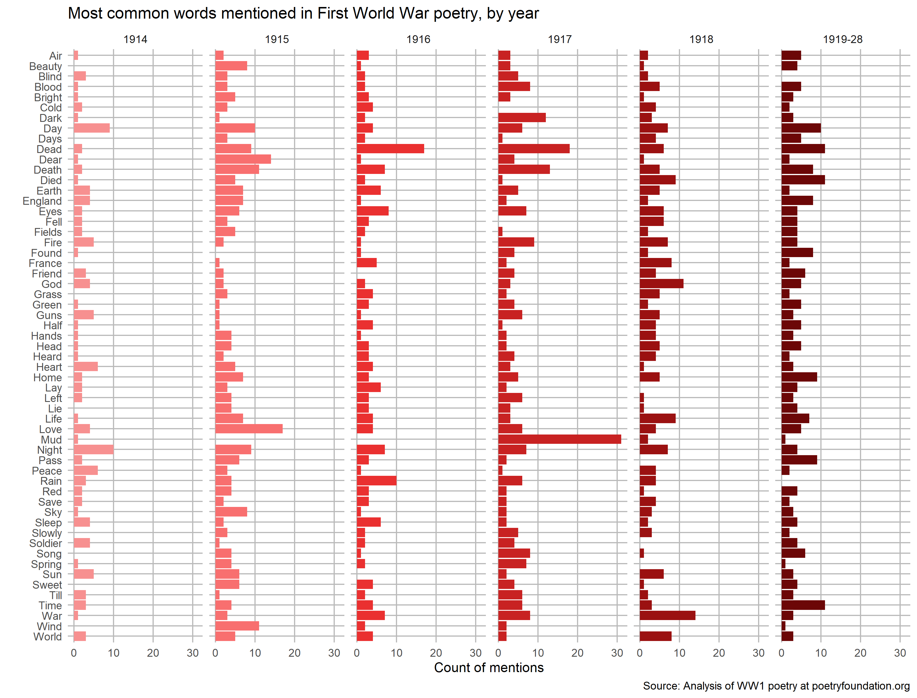
Analysis
Mentions of ‘peace’ peaked in 1914. That year the peace was shattered, yet many soldiers believed the war would be short and peace would return quickly.
When it is peace, then we may view again
With new-won eyes each other’s truer form
And wonder. Grown more loving-kind and warm
We’ll grasp firm hands and laugh at the old pain,
When it is peace. But until peace, the storm
The darkness and the thunder and the rain.Charles Hamilton Sorley, ‘To Germany‘, 1914
Mentions of ‘dead’ peaked in 1916 and 1917. During this time the terrible battles of the Somme and Passchendaele took place. Both battles were notorious for the appallingly muddy conditions, which perhaps explains some of the mentions of ‘mud’ in 1917.
This is the song of the mud,
The pale yellow glistening mud that covers the hills like satin;
The grey gleaming silvery mud that is spread like enamel over the valleys;
The frothing, squirting, spurting, liquid mud that gurgles along the road beds;
The thick elastic mud that is kneaded and pounded and squeezed under the hoofs of the horses;
The invincible, inexhaustible mud of the war zone.Mary Borden, from At the Somme: The Song of the Mud, 1917
Mentions of ‘France’ peaked in 1918, when the end of the war meant the troops could finally go home, many to England, whose mentions peaked following the war.
The half-limbed readers did not chafe
But smiled at one another curiously
Like secret men who know their secret safe.
(This is the thing they know and never speak,
That England one by one had fled to France
Not many elsewhere now save under France).Wilfred Owen, ‘Smile, Smile, Smile’, 1918
Conclusion
I remember studying World War I poetry in English classes for my GCSEs at school. Back then, we went into so much detail that it was difficult to appreciate them for the works of literature that they are.
With this textual analysis approach in R, we can get a different insight to learn what the men and women of the time were thinking when they wrote of the horrors of the First World War.