Earlier this month Marie Segger, Carlos Novoa and I had a major new project published about different rail speeds between cities around Britain.
We compared the distances between train stations in Britain’s largest cities and found which areas were poorly-served by slow trains.

Our project was picked up by a MP for Plymouth, a city that is quite isolated down in Devon and suffers from relatively poor train connections:
Plymouth has one of the slowest train lines in the country according to a new study today https://t.co/8H5J4lwJkC #plymouth #notsurprised
— Luke Pollard MP (@LukePollard) August 2, 2017
Here is how we did it.
Step 1: create a distance calculator function
There are two formulas in here: one to convert degrees into radians and the other two actually make the distance calculator. The second one is adapted from this blog post (thanks a bunch, BlueMM!)
options(scipen = 999)
deg2rad <- function(deg) {(deg * pi) / (180)}

#distance calculator function
 distanceCalc <- function(lat1, lat2, long1, long2) {

acos(cos(deg2rad(90-lat1)) * cos(deg2rad(90-lat2)) + sin(deg2rad(90-lat1)) * sin(deg2rad(90-lat2)) * cos(deg2rad(long1 - long2))) * 3958.756

}
We can now calculate the distance between any two latitude and longitude pairs using this function.
Step 2: Upload the stations
I should point out at this point that the distance calculator only works out straight-line (as the crow flies) distances.
It’s a limitation of this technique because trains don’t travel in absolute straight lines from A to B.
The locations of train stations can be found in the Government’s NAPTAN data under ‘Rail References’ in the zip file.
Unfortunately the location data is in Easting/Northing format. We need it to be in Lat/Long format. That can be done as follows, using Alex Singleton’s work as a template:
library(rgdal)
latlong = "+init=epsg:4326"
coords <- cbind(Easting = as.numeric(as.character(stations$Easting)), Northing = as.numeric(as.character(stations$Northing)))
stations_latlong <- SpatialPointsDataFrame(coords, data = data.frame(stations$StationName,stations$CrsCode),proj4string = CRS("+init=epsg:27700"))
colnames(stations_latlong@coords)[colnames(stations_latlong@coords) == "Easting"] <- "Longitude"
colnames(stations_latlong@coords)[colnames(stations_latlong@coords) == "Northing"] <- "Latitude"
stations_latlong <- spTransform(stations_latlong, CRS(latlong))

> str(stations_df)
> str(stations_df) 'data.frame': 2621 obs. of  5 variables:
$ stations.StationName: Factor w/ 2596 levels "Abbey Wood (London) Rail Station",..: 1801 2160 441 2155 1373 1372 1100 426 83 1512 ...
$ stations.CrsCode    : Factor w/ 2591 levels "AAP","AAT","ABA",..: 1811 2081 431 2036 1469 1370 1219 439 84 1561 ...
$ Longitude           : num  -5.53 -5.48 -5.46 -5.44 -5.44 ...
$ Latitude            : num  50.1 50.2 50.2 50.2 50.2 ...
$ optional            : logi  TRUE TRUE TRUE TRUE TRUE TRUE ...
Now we need to work out which stations we need. The ONS’s built-up areas are the best measure I know of measuring city size. Local authorities in the UK vary greatly in size – the population of the Birmingham council area is about twice that of Manchester even though to most people those cities are similar sizes.
In no particular order, they are:
- Sheffield
- Manchester
- London
- Leicester
- Leeds
- Glasgow
- Coventry
- Birmingham
- Plymouth
- Liverpool
- Edinburgh
- Southampton
- Nottingham
- Newcastle
- Derby
- Bristol
- Stoke-on-Trent
- Hull
- Cardiff
- Bradford
- Portsmouth
Step 3: Calculate each station’s distance from each other
After racking my brains trying to work out how to perform an easy filter for the ones I wanted, I decided it was easier to do every possible combination for all stations and then filter out the superfluous ones.
Again, I couldn’t figure out a way of doing this without using a for loop. If anyone has a simpler, cleaner way, please let me know in the comments!
#create blank data frame to fill in with data
results <- data.frame(NA)
results$distance <- NA
results$station <- NA
results$from <- NA
results <- results[, 2:4]

#i = number of stations
for (i in 1:2621) {
   latitude <- stations_df$Latitude[i]
   longitude <- stations_df$Longitude[i]
   all <- as.data.frame(mapply(FUN = distanceCalc, lat1 = latitude, lat2 = stations_df$Latitude, long1 = longitude, long2 = stations_df$Longitude))
   all$station <- stations_df$stations.StationName
   all$from <- stations_df$stations.StationName[i]
   names(all) <- c("distance","station","from")
   results <- rbind(all, results)
}
There’s an easy way to test whether the distance calculator worked using this radius generator from Free Map Tools.
According to our calculations Birmingham New Street to Cardiff Central station is 88.057 miles.
Let’s see:

There are 1,609.34 metres in a mile, meaning that distance is 141,714 metres. The function seems accurate to about 200m, meaning it is about 99.5 per cent accurate.
Not bad at all.
Here is how a sample of our data looked at this point:
> str(results)
> str(results)'data.frame': 262101 obs. of  3 variables:
$ distance: num  403 397 398 400 399 ...
$ station : Factor w/ 2596 levels "Abbey Wood (London) Rail Station",..: 1801 2160 441 2155 1373 1372 1100 426 83 1512 ...
$ from    : Factor w/ 2596 levels "Abbey Wood (London) Rail Station",..: 2483 2483 2483 2483 2483 2483 2483 2483 2483 2483 ...
Step 4: Filter the stations we’re interested in
Again, I couldn’t see any way of automating this because of the unique station names.
manchester <- results[results$from == "Manchester Piccadilly Rail Station", ]
#etc
Step 5: Get the distances
We stepped away from R here to use OutWit Hub, a scraping program.
Happily The Train Line website has a convenient average time for most major journeys, so we scraped that.
Step 6: Calculate speeds
Going back to GCSE physics:
Speed = distance/time
We have the distances and the times, so dividing one by the other gave us the speeds. Sorting them showed us the fastest to the slowest!
Analysis
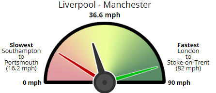
We found that trains to and from London were the fastest in Britain.
In fact the top 22 journeys with the fastest speeds were all two or from the capital.

Towards the other end of the spectrum were journeys that often went across Britain. It’s relatively easy to get up and down the country but going east to west or vice versa takes longer.
The slowest long-distance journey (which we defined as 100 miles or more) was Coventry to Hull, which chugged along at 26mph.
Trains between cities closer together, such as Bradford to Manchester, are likely going to be slower because there’s no distance for the trains to accelerate up to their top speeds.
Obviously the journey times including any waiting times at stations to change trains.
Conclusion
This was the first outing for the distance calculator. We want to use it for other purposes as well in the future.
As it happened, when we were ready to publish there was a furore about the Government’s backtrack (transport journalism is full of puns) on electrifying lines in Wales, the Midlands and the North.
Notably none of these lines were in London, while Crossrail ploughs on, possibly to be followed by Crossrail 2.
Our project exposed how London-centric Britain’s rail network really is.