Before we begin:
Hadley Wickham, the reshape2 package creator, pointed me in the direction of the tidyr package for melting data. I’ll take a look at it after this post.
As promised from before, a look at @hadleywickham‘s reshape2 package and Home Office drugs data #ddj #rstats https://t.co/Q46eUijsaG
— R For Journalists (@rforjournalists) October 18, 2016
Take a look at the thread to see the full conversation.
To recap:
From our last post, we had our data in this format:
> str(london)
'data.frame': 75 obs. of 4 variables:
 $ Drug : Factor w/ 7 levels "Amphetamines",..: 1 4 5 6 7 1 4 5 6 7 ...
 $ Region : chr " London" " London" " London" " London" ...
 $ variable: Factor w/ 15 levels "X2001.02","X2002.03",..: 1 1 1 1 1 2 2 2 2 2 ...
 $ value : num 1.6 14.3 3.6 0.9 4.3 1.9 13.5 2.6 1 3.7 ...
Let’s plot this data:
ggplot(london, aes(y = value, x = variable,
color = Drug, group = Drug)) + geom_line()
Here is the result:

We run into the same problem of overlapping labels that we saw in our dabbling in unemployment data.
We’ll solve it in the same way, by creating some breaks and labels and applying scale_x_discrete. We’ll take every other year and apply labels in the format [YY/YY].
We will also use scale_color_manual to select the colours manually. I want the line representing cannabis to be green and the line representing cocaine to be grey. The others I’ll select from colours that are sufficiently different from green and grey. To select the colours, we use hex codes. These are six-character strings preceded by a hash. Every colour you see on a web page has such a colour code. Go to a website like HTML Color Codes to choose your own. A very useful web browser extension is ColorZilla, which enables you to grab the hex code of any colour you see online.
breaks1 <- c("X2001.02","X2003.04","X2005.06","X2007.08",
"X2009.10","X2011.12","X2013.14","X2015.16")
labels1 <- c("01/02","03/04","05/06",
"07/08","09/10","11/12","13/14","15/16")
ggplot(london, aes(y = value, x = variable,
color = Drug, group = Drug))
+ geom_line(size = 2)
#change colours
+ scale_color_manual(values=c("#FFC300", "#186A3B",
"#5B2C6F","#56B4E9","#B9B1AF"))
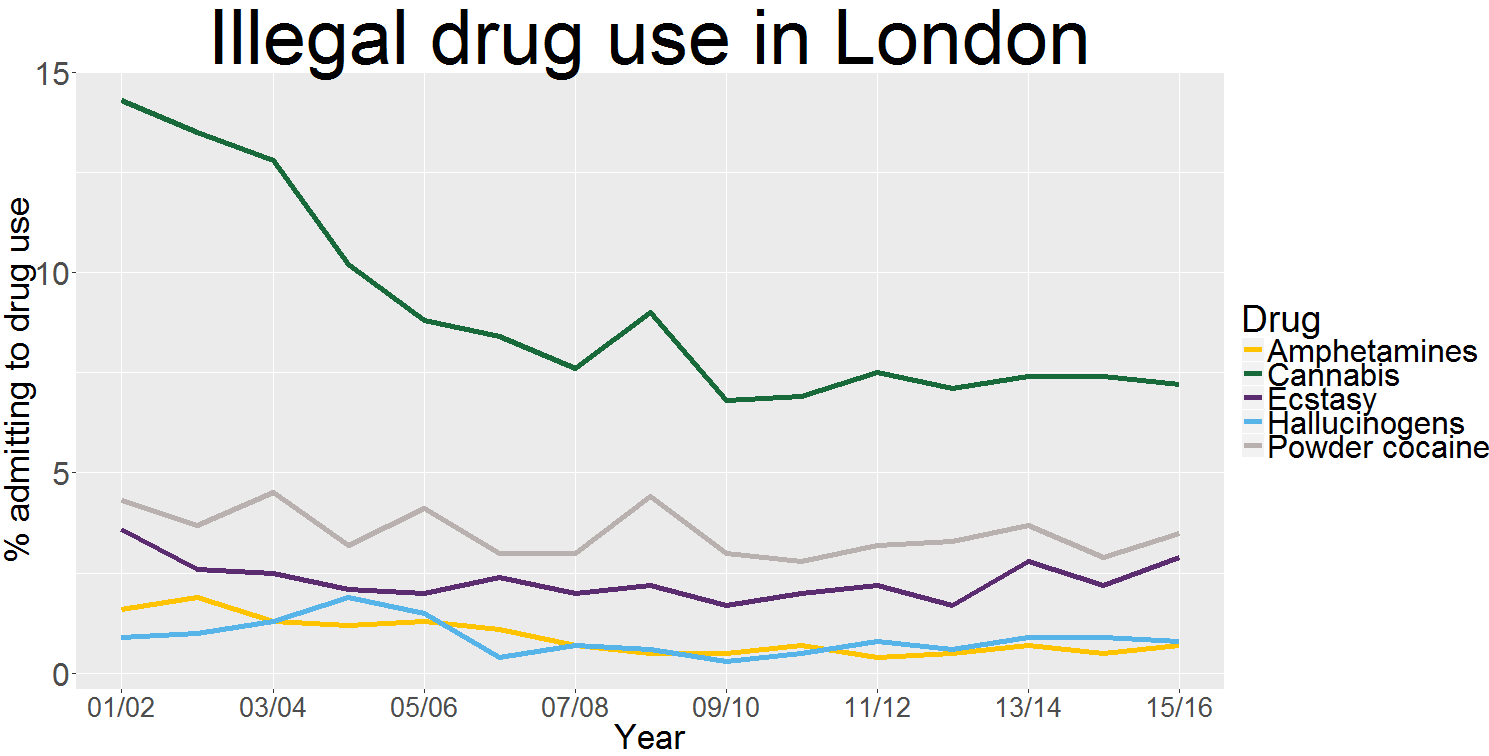
+ ggtitle("Illegal drug use in London")
+ labs(x = "Year", y = "% admitting to drug use")
#add in labels
+ scale_x_discrete(breaks = breaks1, labels = labels1)
#formatting
+ theme(plot.title = element_text(size = 58),
axis.text.y = element_text(size = 24),
axis.text.x = element_text(size = 20),
axis.title = element_text(size =26),
legend.title = element_text(size = 28),
legend.text = element_text(size = 24))
Here’s the result:

Analysis
We can see that cannabis has fallen out of fashion in the capital in recent years. The proportion of Londoners who admitted smoking weed in 2001/02 was close to 15 per cent. Last year that had dropped to 7.2 per cent.
Ecstasy and cocaine on the other hand crept back up again last year.
Let’s look at the South West.
They were the region where the biggest proportion of people admitted illegal drug use last year (10.2 per cent):

Cannabis use declined in the South West in the Noughties but has seen something of a comeback in recent years in the region.
However these five types of drug use in the region were all down year on year.
This concludes our two part post.
We have seen how to use scale_x_discrete again with labels and breaks, as well as how to choose our own colours using hex codes.
We have also met the melt formula. I’ll post soon about the gather function, which I gather is superior.